- Organization
-
IAU Double Star Center
- WDS Description
-
WDS Catalog
- WDS Catalog: Full
- WDS Catalog: 00-05 Hour Section
- WDS Catalog: 06-11 Hour Section
- WDS Catalog: 12-17 Hour Section
- WDS Catalog: 18-23 Hour Section
- WDS Catalog With Precise Last Only
- WDS Catalog As An SQL Database (Original Code, Danley Hsu; Improved Code, Damien Mattei)
- WDS With Constellation And Bayer/Flamsteed Designation (When Applicable) Appended
- Format Of The Current WDS
- Notes File For The WDS
- References And Discoverer Codes
-
WDS Supplemental Catalog
- WDS Supplemental Catalog: Explanatory file
- WDS Supplemental Catalog: Summary
- WDS Supplemental Catalog: 00-05 Hour Section (All Data)
- WDS Supplemental Catalog: 06-11 Hour Section (All Data)
- WDS Supplemental Catalog: 12-17 Hour Section (All Data)
- WDS Supplemental Catalog: 18-23 Hour Section (All Data)
- WDS Supplemental Catalog: Format Of Files
- IAU Commission G1
-
Sixth Catalog Of Orbits Of Visual Binary Stars
- Full Page
- Introduction
- Orbit Grading Method
- Description Of The Catalog
- Catalog statistics
- Acknowledgments And References
- Orbital Elements: Html
- Orbital Elements: Text
- Orbital Elements: SQL
- Ephemerides:Html
- Ephemerides:Text
- Notes:Html
- Notes:Text
- References:Html
- References:Text
- Orbital Elements: Frame Version
- Formats Of Elements And Ephemerides Files
- Calibration Candidates
- Top 25 Orbit Calculators
- Master File Database
- Catalog Of Rectilinear Elements
- Fourth Catalog Of Interferometric Measurements Of Binary Stars
- The Delta-M Catalog
- IERS ICRS Center
- IVS (VLBI) Analysis Center
- IVS (VLBI) Analysis Center for Source Structure
-
Data Products
- Overview
-
IAU Double star center
- Overview
-
WDS Catalog
- WDS Catalog: Full
- WDS Catalog: 00-05 Hour Section
- WDS Catalog: 06-11 Hour Section
- WDS Catalog: 12-17 Hour Section
- WDS Catalog: 18-23 Hour Section
- WDS Catalog With Precise Last Only
- WDS Catalog As An SQL Database (Original Code, Danley Hsu; Improved Code, Damien Mattei)
- WDS With Constellation And Bayer/Flamsteed Designation (When Applicable) Appended
- Format Of The Current WDS
- Notes File For The WDS
- References And Discoverer Codes
-
WDS Supplemental Catalog
- WDS Supplemental Catalog: Explanatory file
- WDS Supplemental Catalog: Summary
- WDS Supplemental Catalog: 00-05 Hour Section (All Data)
- WDS Supplemental Catalog: 06-11 Hour Section (All Data)
- WDS Supplemental Catalog: 12-17 Hour Section (All Data)
- WDS Supplemental Catalog: 18-23 Hour Section (All Data)
- WDS Supplemental Catalog: Format Of Files
-
Sixth Catalog Of Orbits Of Visual Binary Stars
- Full Page
- Introduction
- Orbit Grading Method
- Description Of The Catalog
- Catalog statistics
- Acknowledgments And References
- Orbital Elements: Html
- Orbital Elements: Text
- Orbital Elements: SQL
- Ephemerides:Html
- Ephemerides:Text
- Notes:Html
- Notes:Text
- References:Html
- References:Text
- Orbital Elements: Frame Version
- Formats Of Elements And Ephemerides Files
- Calibration Candidates
- Top 25 Orbit Calculators
- Master File Database
- Catalog Of Rectilinear Elements
- Fourth Catalog Of Interferometric Measurements Of Binary Stars
- The Delta-M Catalog
- FRIDA
- 24 Hour Sessions
- UT1-UTC
- Global Solutions
Sixth Catalog of Orbits of Visual Binary Stars (WDS-ORB6)
Note: The following description is adapted from a paper by Hartkopf et al. (2001 AJ 122, 3472.)
The Sixth Catalog of Orbits of Visual Binary Stars continues the series of compilations of visual binary star orbits published by William Finsen, Charles Worley, and Wulff Heintz from the 1930s to the 1980s. As of 27 July 2017 the new catalog included 2,739 orbits of 2,656 systems. All orbits have been graded as in earlier catalogs, although the grading scheme was modified as of the Fifth Catalog to be more objective. Ephemerides are given for all orbits, as are plots including all associated data in the Washington Double Star (WDS) database. A subset of orbits potentially useful for scale calibration is also presented.
The Sixth Catalog of Orbits of Visual Binary Stars (henceforth Sixth Catalog ; Hartkopf et al. 2001a) continues the series of compilations of visual binary star orbits previously published by Finsen (1934, 1938); Worley (1963); Finsen & Worley (1970); Worley & Heintz (1983, henceforth Fourth Catalog ); and most recently by Hartkopf, Mason, & Worley (2001b, henceforth Fifth Catalog ).
The 3+ decades since publication of the Fourth Catalog have seen revolutionary changes in the field of visual double star work, primarily through the advent and maturation of interferometry. Speckle interferometry, especially on large telescopes, can produce astrometric results of very high accuracy (down to milliarcsecond level), even for systems much closer and of shorter period than those available to micrometry and other visual techniques. Although the speckle technique has been known since 1970, it did not produce data in significant quantity until about 1975; at the time of publication of the Fourth Catalog only a handful of orbits had been calculated in which speckle played much of a role. Now, however, speckle interferometry is a mature field, and nearly all orbits published since the 1980's have included speckle results, some exclusively. Long-baseline interferometry [e.g., Mark III (cf., Pan et al. 1990) and the Navy Precision Optical Interferometer (NPOI; cf., Hummel et al. 1998)] is now perhaps in a similar degree of maturation as was speckle in 1983; an increasing number of binaries once exclusively the "property" of spectroscopists are now the targets of multi-aperture telescope arrays. Indeed, the distinction between the spectroscopic and visual regimes will largely disappear in the coming decades, as the magnitude sensitivity of these new interferometers improves. Catalogs such as this will have to evolve as well; as spectroscopic + visual "combined solutions" go from being rare to commonplace, the argument for publishing only a subset of a binary's elements will grow increasingly artificial. For the present, however, information on combined solutions is relegated to a notes file.
A major consideration in the production of a new catalog is the determination of grades for each orbit. The Fourth Catalog grading scheme was based on orbital coverage, number of observations, and their overall quality, and presented on a numerical scale (1=definitive to 5=indeterminate - see Figure 1 for examples) based on the accumulated experience of the authors and their qualitative assessment of individual observers. (It should be noted that Worley and Heintz had some six decades' worth of combined experience at the time they published the Fourth Catalog ; these two gentlemen also rank as the third and second most prolific binary star observers of all time.) While useful for judging the reliability of a given orbit, this scheme was rather subjective, and therefore difficult to duplicate by catalogers having less experience. For the Fifth Catalog we attempted to devise a more objective grading scheme, based on the same information as that available to Worley and Heintz. This same grading scheme is used for the Sixth Catalog as well.
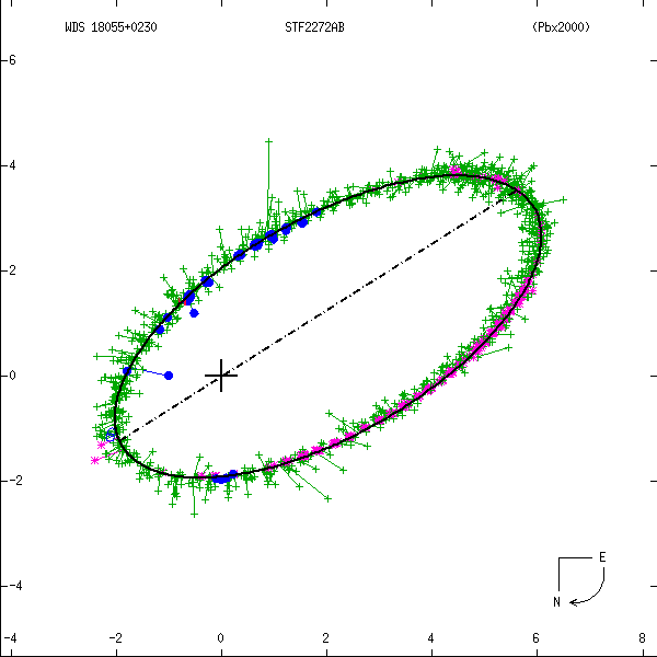

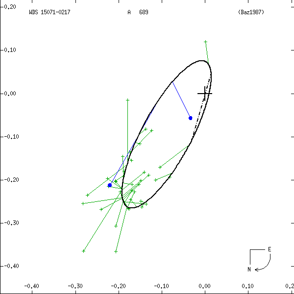
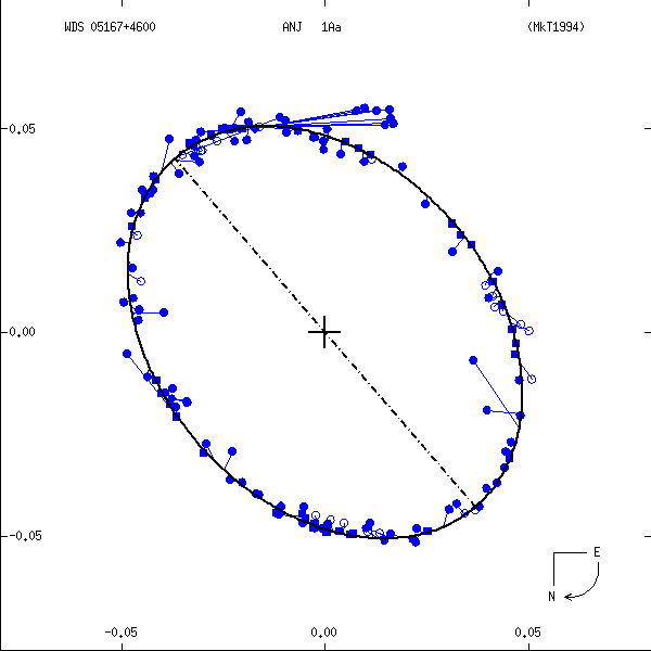
Figure 1: Two examples each of grade 1 (left) and grade 5 (right) orbits. Factors used in determining these grades are discussed below. In these and all other orbit figures in this catalog, green plus signs indicate visual (micrometric) observations, violet asterisks photographic measures, and blue symbols various interferometric techniques (open circles, filled circles, and filled squares for eyepiece interferometry, speckle or other single-aperture techniques, and multi-aperture techniques, respectively). Finally, a red "H" or "T" indicates a measure from Hipparcos or Tycho. The dot-dash line indicates the line of nodes. Scales are in arcseconds, and the curved arrow at lower right indicates the direction of orbital motion.
Evaluating the Observations
In order to determine rms residuals, we first must determine relative weights to be assigned to each observation. The following factors were considered:
- telescope aperture
- binary separation
- magnitude and magnitude difference: Since we are mainly interested in relative weights to be assigned for observations of a given binary, these factors are presumed constant and we have ignored them.
- "number of nights": Some observers publish individual measures, while others average 2 or more into means. A simple sqrt( N ) term handles this.
- expertise of the observer: This is the most difficult factor to evaluate. Accuracy should improve with experience, but may decrease as, for example, a visual observer's eyesight deteriorates with age (some observers produced measurements for 40, 50, and even 70 years). We have ignored this age factor for the present, however.
- other factors, such as systematic errors in a given piece of equipment, quality of the scale calibration, seeing conditions at a given site, etc.: These are ignored as separate factors, but obviously are part of the "observer expertise" factor.
The best method we really have for evaluating the quality of an observation is to see how it compares with others. In practical terms this means we examine the size of the orbit residuals it gives. Here we unfortunately are stuck with a bit of a circular argument: in order to assign weights to observations we must compare them to orbits. Yet in order to determine those orbits in the first place we must assign weights to the observations! The way in which we chose to minimize this problem was by sheer force of numbers - by examining many well-observed binaries whose orbits are generally acknowledged to be of high quality.
All grade 1 and 2 orbits from the Fourth Catalog were examined, together with all more recently published orbits and numerous long-period orbits (such as GRB 34 in Figure 1). This last group was included in order to evaluate observers of wider systems. Many of these systems show small orbit residuals over the covered orbit arc, although the lack of phase coverage earns them a poor grade. From ~750 orbits and over 100,000 observations initially examined, some 450 orbits and ~66,000 observations were chosen for evaluation of observer weights.
Since the number of "degrees of freedom" is large, we simplified the problem in two ways:
- Since binary resolution is a function of telescope aperture, we remove this complication by scaling separation to the Rayleigh limit of the telescope used ( rho_lim ~ L / D , where L is the wavelength and D is the telescope diameter. Assuming L = 550nm, rho_lim = 0.136/ D , for rho_lim in arcseconds and D in meters).
- Different observing techniques - micrometry, photography (including conventional CCD observations), and interferometry (plus adaptive optics, satellite observations, and other high-resolution techniques) - were evaluated separately. All data for a given technique were first studied, then relative weights for observers using that technique determined.
Figures 2 and 3 illustrate some of our initial findings on accuracy versus separation for the different techniques. Both theta and rho residuals show obvious dependence on separation. The long-known fact that separations of very close systems are systematically overestimated is also apparent, especially in Figure 2a. Assuming (d rho / rho )^(-2) gives a reasonable estimate of the relative weight of an observation, we fit a polynomial to (d rho / rho )^(-2) versus rho / rho_lim for each technique to determine this first weighting factor as a function of separation and telescope aperture.
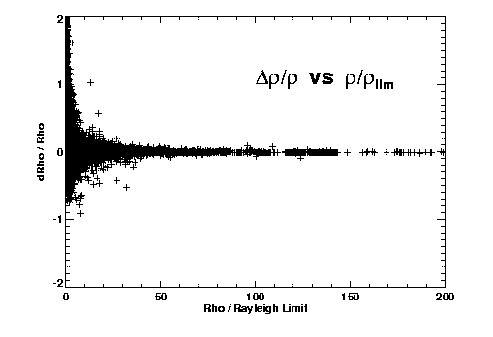
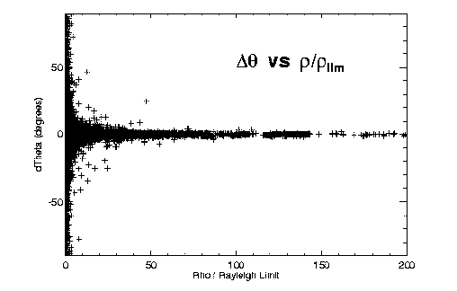
Figure 2: O-C errors in (left) relative separation and (right) position angle, versus separation (scaled to each telescope's Rayleigh limit).
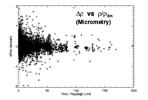
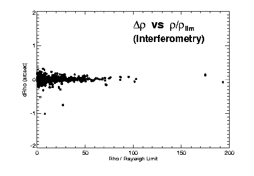
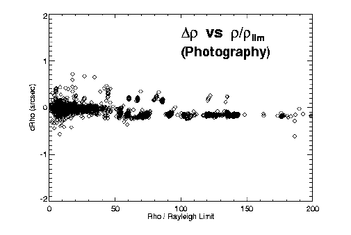
Figure 3: O-C separation errors versus separation, for (left) visual, (center) interferometric, and (right) photographic observing techniques. The relative accuracies of the three techniques are apparent.
As a second step, we wish to determine the relative qualities of each observer who uses a given technique. We do this by removing the overall error versus separation fit derived above, then determining rms residuals for each observer. Observers having too few measures for individual weighting are averaged together. Relative weights for each observer are then defined as the inverse square of their rms residual (with the weighted mean weight for each technique scaled to 1). We find:
- Visual observers received a wide range in relative weight, from about 0.1 to 4.5. It must be noted that this is not really a measure of an observer's competence; a person who only looks at bright, wide, low zenith-distance, small d m pairs will tend to receive a better grade than does someone who pushes his instrument to its limits in magnitude, d m , etc. These more difficult observations are usually the more important, however.
- Photographic observers were of fairly uniform quality. Observers having significant numbers of measures ranged in relative weight from about 0.5 to 1.4, while the observers making smaller contributions received a weight of 0.3. Since photographic techniques are presumably somewhat more objective than visual measurement, this finding seems reasonable.
- Eyepiece interferometry tends to get rather low marks (0.01 to 0.3) compared to other interferometric techniques. Speckle and other single-aperture techniques garnered weights of 0.02 to 1.4, with the larger speckle efforts generally receiving the higher weights. The Mark III received a comparable weight of about 0.9. NPOI received a very high weight (13.3), but this is rather misleading, as the number of measures is small and the separation regime of this instrument is such that this is largely an indication of internal consistency.
As mentioned earlier, the third factor is simply the sqrt( N ) term which gives higher weight to normal points averaged from more than one observation. Finally, a few measures in the WDS are flagged as being uncertain or of poor quality. The term W_quality , usually assigned a value of unity, is reduced by half for such measures. The overall weight of a given observation, then, is determined by the product of these four terms:
W = W _technique ( rho , aperture) * W _observer * sqrt( N _measures) * W _quality
UPDATE:The method for deriving weights of individual measures was extensively modified in 2017 September, largely in response to the much greater quantity of CCD and interferometric data now available, and the corresponding decrease in the use of micrometry. Rather than using only a few technique categories and separate "quality" assessments of many individual observers, weights were determined for 18 different techniques, based on the technique codes used in the WDS. These technique categories are as follows:
- A
- C
- E (mostly E2)
- Eu
- H (mostly Hf,Ht,Hw)
- Hh
- J
- K
- M (dates 1750-1829)
- M (dates 1830-1849)
- M (dates 1850-present)
- P (mostly Pa)
- Po
- S/I (tel 0.00 - 1.49m)
- S/I (tel 1.50 - 2.49m)
- S/I (tel 2.50 - 99.99m)
- T
- misc (other techniques)
Scale residuals (drho/rho) were determined for 90,000+ measures (based on 493 well-determined orbits and 933 linear fits). Relative weights for each technique were then derived by comparing mean residuals between, for example, CCD and AO, for all orbit or linear pairs having both types of data in common. For this comparison, only measures with separations well above the Rayleigh limit for a given telescope/filter combination were utilized.
Micrometry data were subdivided into various date ranges (since the earliest micrometry measures are known to be of significantly lower quality than later measures). After some experimentation, the date ranges given in the above list were found to be reasonable subdivisions for the technique. In a similar manner, speckle interferometry data were subdivided by telescope aperture, and the three aperture ranges given above were found to be appropriate. Subcategories for space-based (code H) and wide-field imaging (technique E) were checked, as well.
Results are as one might expect. Assuming a mean weight for CCD measures of 1.0, post-1850 micrometry has a comparative weight of about 0.1, with the earliest micrometry measures only 0.01. Large-aperture speckle measures have a relative weight of just over 10, and long-baseline interferometry yields a relative weight on this scale of about 140.
As mentioned above, measures obtained at separations near an instrument's Rayleigh limit will typically be of much lower quality than those obtained at larger separations. In order to determine relative weight for a given technique as a function of separation, residuals in each technique category were converted to weights and sorted by separation (in "rayleighs", as described above). Running mean weights were determined, and quadratic or cubic fits made to each running mean. These were finally scaled to a maximum weight of one. As expected, these weights begin at a value of zero at zero separation, and rise to a value of 1.0 at some 10s of "rayleighs" in separation.
As described earlier, the overall weight of a given observation, then, is determined by the product of four terms, now slightly modified to:
W = W _technique * W _separation * sqrt( N _measures) * W _quality
One additional modification should be noted. Speckle obserations made at separations beyond the size of the isoplanatic patch will be of degraded quality; W_quality is therefore set to 0.5 for any speckle measure made at a separation greater than 3 arcseconds.
Evaluating the Orbits
Worley & Heintz used the following criteria for each orbit grade (as quoted from the Fourth Catalog ):
- 1 = Definitive.
- Well-distributed coverage exceeding one revolution; no revisions expected except for minor adjustments.
- 2 = Good.
- Most of a revolution, well observed, with sufficient curvature to give considerable confidence in the derived elements. No major changes in the elements likely.
- 3 = Reliable.
- At least half of the orbit defined, but the lesser coverage (in number or distribution) or data consistency leaves the possibility of larger errors than in Grade 2.
- 4 = Preliminary.
- Individual elements entitled to little weight,and may be subject to substantial revisions. The quantity 3 log( a ) - 2 log( P ) should not be grossly erroneous. This class contains: orbits with less than half the ellipse defined; orbits with weak or inconsistent data; orbits showing deteriorating representations of recent data...
- 5 = Indeterminate.
- The elements may not even be approximately correct. The observed arc is usually too short, with little curvature, and frequently there are large residuals associated with the computations.
How can these grades be determined in an objective manner? We evaluated as many of the 928 orbits in the Fourth Catalog as possible, as follows. We extracted from the WDS the ~100,000 observations made of these objects through 1982 (i.e., the same data available to Worley and Heintz for their evaluations). After removing orbits without grades, plus a few problematic orbits and obviously erroneous measures, we were left with 901 orbits and 93,775 observations. We then determined the following statistical factors for each system:
- weighted rms residual in separation (d R )
- weighted rms residual in relative separation (i.e., d R / R )
- theta coverage: measures were sorted in order of theta , then the rms difference in angle [i.e., theta (n) - theta (n-1)] was calculated
- maximum "gap" in theta : also from above theta sort
- phase coverage: calculated from period ( P ) and periastron epoch ( T ), then sorted and rms differences determined as done with theta
- maximum "gap" in phase (Why analyze both theta and phase coverage? While both position angle and phase are equivalent for a circular, face-on orbit, position angle coverage becomes increasingly meaningless for inclinations approaching 90 degrees, while uniform phase coverage may undersample periastron passage for a high-eccentricity orbit.)
- number of revolutions from first to last observation
- total number of observations
Some of our results are shown in Figure 4. Data for each grade are spread over three lines in order to more easily see individual points. Means are listed below the data for each grade, with vertical lines indicating mean and 1 sigma values. "Outliers" (removed from the statistics) are plotted in smaller symbols.
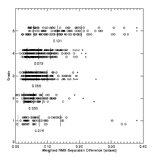

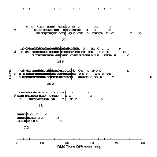
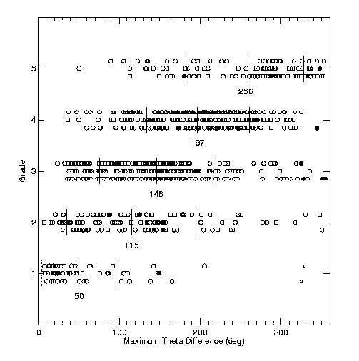
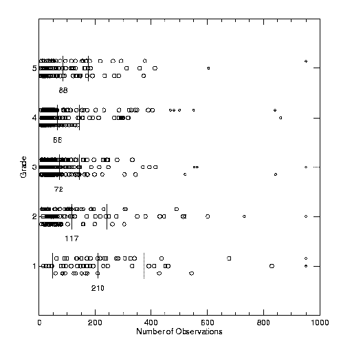
Figure 4: Fitting WH4 grades to rms residuals and other factors, as described in the text.
As is apparent in both the orbit examples in Figure 1 and the Figure 4 results, no one factor alone is sufficient for determining the grade. For example, some poorer orbits show very small separation residuals (as evidenced by the turnover in the rms d R / R plot for grades 4 and 5); the extremely long period (and resulting poor orbit coverage) determines their grade. Others have shorter periods, thus good coverage, but are close and difficult to measure, yielding large separation residuals.
Simple polynomial fits were made between each set of means and their corresponding grades, and the best fit to the Fourth Catalog grades was found by averaging results for the number of observations, the number of revolutions, the maximum angle and phase gaps, and the weighted rms separation residual. New grades were then calculated for each of the 901 orbits based on all these factors; Figure 5 illustrates the degree of correlation between our new, "objective" grades and the Fourth Catalog originals. Some 98% of the grades matched to within one grade level. A check of those systems where our grades disagreed by more than 1 grade found that in nearly all cases the Fourth Catalog grades appeared to be in error. It therefore appears that our quantitative method for grading orbits gives a reasonably good match to Worley & Heintz' originals.
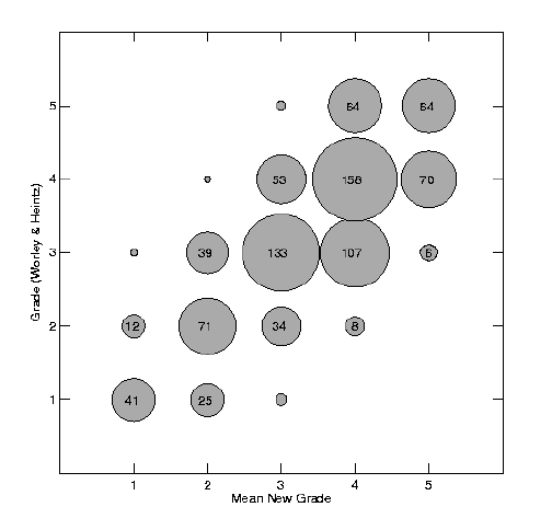
Figure 5: Comparison of grades determined by the method described here with those determined by Worley & Heintz. Circle sizes are scaled to the corresponding number of orbits with these grades; the numbers themselves are given inside all but the smallest circles, where N is only 1 or 2.
One last adjustment was made before grades were determined for all orbits. Thanks to the higher astrometric accuracy achievable by interferometric techniques, we now have the ability to determine orbital elements with higher accuracy than previously considered possible. Since an old "grade 1" orbit may no longer be considered definitive , we have applied a "grade deflation" factor by modifying our polynomial fits somewhat. The factors we applied are as follows:
old grade 1 --> new grade 1.4
old grade 2 --> new grade 2.3
old grade 3 --> new grade 3.2
old grade 4 --> new grade 4.1
old grade 5 --> new grade 5.0
It is worth noting that combined astrometric/spectroscopic solutions are graded only on the number, quality, and distribution of their differential astrometric measures. These solutions typically have P , T , e , and w (or at least a subset of these elements) known to higher accuracy than is reflected in only the visual data. The quality of a combined solution orbit is therefore higher than the grade indicates, although the extent of the improvement depends on the quality of the spectroscopic data, the evaluation of which is beyond the scope of this catalog. The fact that an orbit is a combined solution is certainly taken into consideration when evaluating which orbit of a given pair is considered "best".
A handful of orbits could not be graded, due to a lack of rho and theta measures in the WDS. The first class of these are the few interferometric binaries observed by the Mark III or the Palomar Testbed Interferometer (c.f., Boden et al. 1999) for whom only visibilities were published. These orbits, given a grade of "8" in the catalog, are usually of quite high quality. More common are astrometric orbits, which receive a grade of "9"; these orbits tend to give rather poor fits to any later resolved measures.
A final note: we do not consider this grading method optimum; a visual inspection of competing orbits is still necessary if their grades are within a few tenths of each other. Other schemes, such as the "efficiency" technique of Eichhorn (c.f., Eichhorn & Cole 1985), may be superior and worth investigating. For the present, however, we think this method gives reasonably reliable results.
(Note: All observer weights were reevaluated in March 2004, and all orbits were regraded and new figures generated on a regular basis to reflect measures recently added to the WDS. The reevaulation weights led to minor changes for most orbits - typically 0.0 to 0.2 grades - but the inclusion of new data has occasionally resulted in major revisions of grades for individual systems, as might be expected.)
The "master file" for the Sixth Catalog includes all sets of orbital elements in the Fourth Catalog , as well as all subsequently published orbits either tabulated by Worley or found through searches of the literature from 1980 through the present. Several older catalogs, including those of See (1898), Lewis (1906), and Finsen & Worley (1970) have been added for historical purposes; others are being incorporated as time permits. This file included 8,406 orbits of 2,656 systems as of 27 July 2017. All orbits are graded, and only those judged of highest grade for each system are included in the published Sixth Catalog . If two orbits for a given system are judged to be of nearly identical quality, the earlier-published orbit is usually chosen for the catalog (unless the later orbit also includes formal errors to the elements). A few systems are found to have two very different sets of orbital elements which yield comparable grades; in these cases both orbits are included. These "special cases" bring the total number of orbits in the current Sixth Catalog to 2,739.
Names and orbital elements for a given system are tabulated on two lines, with a blank line separating each orbit for ease in reading. A text version of the catalog (one line per orbit) is also available, as described in the format description page. Columns in the main catalog are as follows:
Line 1:
- Epoch-2000 coordinates, usually given to 0.01s accuracy in right ascension and 0.1" in declination. Most coordinates were extracted from the Tycho-2 catalog.
- Washington Double Star (WDS) designation. Many of these coordinates (given to 0.1m and 1') were generated by precessing lower precision B1900 positions to J2000; therefore the WDS designations may vary slightly from the coordinates in column 1.
- Discoverer designation and components involved. If no components are listed, the orbit is of the AB pair.
- HD (Henry Draper catalog) number.
- Magnitude of the primary component. Codes ">" and "<" preceding the magnitude indicate the value is an upper or lower limit. Codes "v" or "k" following the value indicates a star of variable magnitude or a K-band magnitude.
- The period ( P ), followed by code indicating units: "c" = centuries, "d" = days, "h" = hours, "m" = minutes, "y" = years.
- The semi-major axis ( a ), followed by code indicating units: "a" = arcseconds, "m" = milliarcseconds, "u" = microarcseconds.
- The inclination ( i ), in degrees.
- The node ( Omega ), in degrees. An identified ascending node is indicated by an asterisk following the value.
- The time of periastron passage ( T ), followed by code indicating units: "d" = Julian date, with first two digits truncated (i.e., JD-2400000), "m" = modified Julian date (JD-2400000.5), "y" = fractional Besselian year.
- The eccentricity ( e ).
- The longitude of periastron ( w ), in degrees, reckoned from the node as listed.
- Equinox, if any, to which the node refers.
- The grade (to nearest integer), as previously discussed.
- A link "N" to any notes for this system.
- A link "P" to a figure illustrating the orbit and all data for this object currently tabulated in the WDS database. Symbols used in these figures are as in Figure 1.
- A link "E" to appropriate entries in the ephemeris file.
- A code for the reference (usually based on the name of the first author and the date of publication), with a link to a reference file.
Line 2:
- ADS (Aitken Double Star catalog) number.
- Hipparcos number.
- Magnitude of the secondary component. Codes are as described for the primary.
- Published formal errors in P . Units are the same as for P .
- Published formal errors in a . Units are the same as for i .
- Published formal errors in i .
- Published formal errors in Omega .
- Published formal errors in T . Units are the same as for T .
- Published formal errors in e .
- Published formal errors in w .
- The date of the last observation used in the orbit calculation, when given.
Columns in the ephemeris file are as follows:
- The WDS designation, as above.
- The discoverer designation, as above.
- The orbit grade, as above.
- The reference code, as above.
- Predicted values of theta and rho for the years 2005-2009.
CALIBRATION SYSTEMS
A subset of systems from the Sixth Catalog was prepared in answer to requests for lists of binaries which might be used for scale calibration purposes. Stars initially picked for this list included most of the "grade 1" orbits; these are systems having many observations (usually covering more than one orbital revolution), good phase coverage, and small separation residuals. These tend to be closer, shorter-period systems, in some cases resolvable only by large telescopes or multi-aperture interferometers. In order to provide calibrators for smaller instruments, a similar number of wider, long-period systems were chosen as well. Orbital coverage for these wide systems is incomplete, so most were given grades of only 4 or 5; however, since orbital motion is slow, the quoted elements should predict the stars' motions quite well for many years into the future.
This subset of the Sixth Catalog presently includes 81 orbits of 80 systems. As in the main catalog, figures are included in order to allow the user to visually inspect each orbit's quality prior to use. An expanded set of ephemerides has also been generated, giving predicted separations and position angles with finer time resolution than in the main catalog (although these ephemerides will obviously still be of little use for very short-period systems).
Note that all "calibration candidate" orbits are not of the same quality. Before adopting a set of elements it is recommended that users examine the elements, figures, etc. carefully to check whether that orbit appears to be of proper scale and sufficient quality for their purposes. Also, using measurements of double stars to calibrate the measurement of other double stars is certainly circular (or, if you will, Keplerian). We strongly advocate the use of other absolute calibration techniques such as a slit mask (cf., McAlister et al. 1987, Hartkopf et al. 1997, Douglass et al. 1997) or at least star trails (for east-west orientation) if at all possible. When double stars are necessary for scale calibration, the set provided should be adequate; however, the measures determined will only be as accurate as the calibration systems used. The use of these systems for identification of higher-order motions or submotions is discouraged.
Various statistical comparisons of the Sixth Catalog can be made, both with earlier orbit catalogs and with itself. Figures 6 and 7 (below) show the distribution of orbits with grade and period for the current catalog, together with the corresponding numbers for four earlier catalogs.
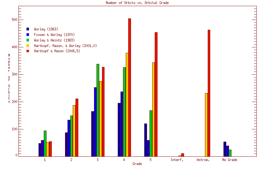
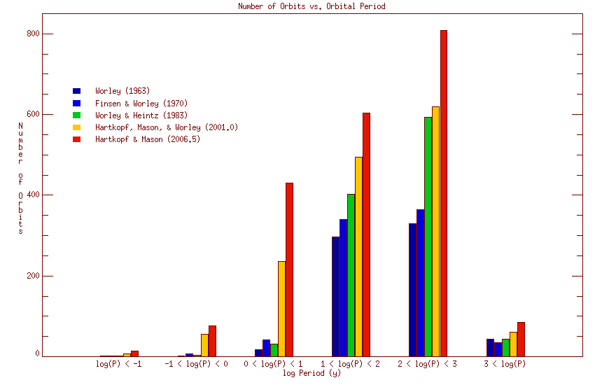
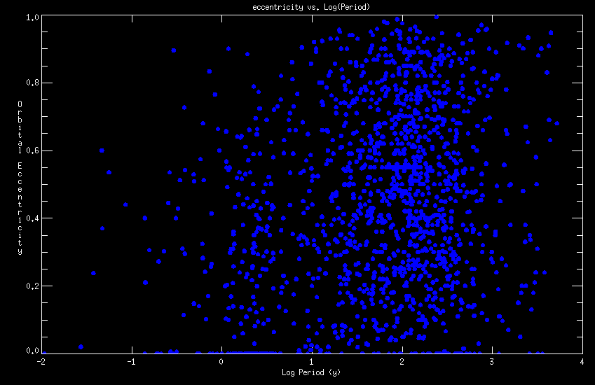
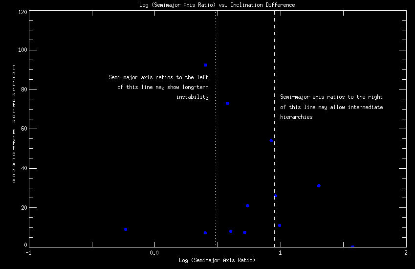
Figure 8 (above) shows a plot of log( P ) versus e for the orbits in the Sixth Catalog . The dramatic circularization seen in similar plots for spectroscopic binaries is not seen in resolved binaries, due to their longer periods.
Finally, Figure 9 (above) is a plot of [Periastron_(outer binary) / Apastron_(inner binary)] versus |i_(outer binary) - i_(inner binary)| for the twenty hierarchical systems with visual orbits determined for both hierarchies. Harrington (1992) quantified a value of 3 for the ratio of periastron(outer binary) to apastron(inner binary) of the inner binary as the critical factor for long-term stability (assuming equal mass companions). Hierarchies to the left of the dotted line may demonstrate long-term instabilities, while those to the right of the dashed line have ratios that may allow intermediate hierarchies.
Systems which are mildly interacting may show a tendency towards co-planarity, so the tendency of smaller inclination differences having smaller period ratios is not surprising. Of the five systems lying between the dotted and dashed lines:
- 02291+6724 = CHR 6Aa + STF 262Aa-B : Both orbits are of grade 5 and the ratio here is suspect.
- 06003-3102 = HU 1399AB + HJ 3823AB-C : this one is the closest to the line and the incomplete orbital coverage of the wider system may be the culprit.
- 08592+4803 = HU 628BC + HJ 2477A-BC : the orbit for the wider system is highly suspect. There seems to be a systematic drift in the O-C values for this orbit and it may not be even a physical association.
- 23019+4220 = BLA 12Aa + WRH 37Aa-B : The short-period orbit is based on only five data points (one of those with a large residual) and needs more data.
- 23393+4543 = CHR 149Aa + 3A 643Aa-B : Also suffering from a paucity of data, the short-period system here has four differential measures and needs more data, too.
Thanks foremost to the U.S. Naval Observatory for five decades' worth of support for the USNO double star observing program and the Washington Double Star Catalog and related products. Thanks also to the late Drs. Wulff Heintz and William Finsen, without whose efforts this series of catalogs would never have existed. This catalog has made use of the SIMBAD database.
We dedicate this catalog to the memory of Charles Edmund Worley, our colleague and friend.
REFERENCES
- Boden, A.F. et al. 1999, ApJ 527, 360
- Douglass, G.G., Hindsley, R.B., & Worley, C.E. 1997, ApJS, 111, 289
- Eichhorn, H. & Cole, C.S. 1985, Celestial Mechanics 37, 263
- Finsen, W.S. 1934, Union Obs. Circ. 4, 23
- Finsen, W.S. 1938, Union Obs. Circ. 4, 466
- Finsen, W.S. & Worley, C.E. 1970, Republic Obs. Circ. 7, 203
- Harrington, R.S. 1992, "A Review of Dynamical Studies of Multiple Stars", Complementary Approaches to Double and Multiple Star Research , ASP Conference Series, Vol. 32, IAU Colloquium 135, H.A. McAlister and W.I. Hartkopf, Eds., p. 212
- Hartkopf, W.I. & Mason, B.D., & Worley, C.E. 2001a, Sixth Catalog of Orbits of Visual Binary Stars , http://www.ad.usno.navy.mil/WDS/orb6/orb6.html
- Hartkopf, W.I., Mason, B.D., & Worley, C.E. 2001b, Fifth Catalog of Orbits of Visual Binary Stars , http://www.ad.usno.navy.mil/WDS/orb5/hmw5.html
- Hartkopf, W.I., McAlister, H.A., Mason, B.D., ten Brummelaar, T., Roberts, L.C., Jr., Turner, N.H., & Wilson, J.W., 1997, AJ, 114, 1639
- Hummel, C.A., Mozurkewich, D., Armstrong, J.T., Hajian, A.R., Elias, N.M., & Hutter, D.J. 1998, AJ 116, 2536
- Lewis, T. 1906, MemRAS 56
- McAlister, H.A., Hartkopf, W.I., Hutter, D.J., & Franz, O.G. 1987, AJ, 93, 688
- Pan, X.P., Shao, M., Colavita, M.M., Mozurkewich, D., Simon, R.S., & Johnston, K.J. 1990, ApJ, 356, 641
- See, T.J.J. 1898, Evolution of Stellar Systems, v1
- Worley, C.E. 1963, Pub. U.S. Naval Obs. 18, pt. 3
- Worley, C.E. & Heintz, W.D. 1983, Pub. U.S. Naval Obs. 24, pt. 7